Auto Encoders

Auto Encoders

Auto encoders are one of the unsupervised deep learning models. The aim of an auto encoder is dimensionality reduction and feature discovery. An auto encoder is trained to predict its own input, but to prevent the model from learning the identity mapping, some constraints are applied to the hidden units.

The simplest form of an auto encoder is a feedforward neural network where the input $x$ is fed to the hidden layer of $h(x)$ and $h(x)$ is then fed to calculate the output $\hat{x}$. A simple auto encoder is shown in Fig1.

Fig1. - A simple Autoencoder.

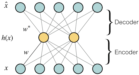
The following equation can describe an autoencoder:

$$\hat{x} = O(a(h) ) = Sigmoid ( c + w^{*} h(x)),$$

$$h(x) = g(a(x)) = Sigmoid (b + Wx),$$

where $a$ is a linear transformation and both $O, g$ are activation functions.

The autoencoder tries to reconstruct the input. So if inputs are real values, the loss function can be computed as the following mean square error (MSE):

$$l = \frac{1}{2} \sum_{k=1}^N (x_{k} - \hat{x_{k}})^2,$$

where $N$ is the number of examples. But if the inputs are binary, we can define our loss function as a binary cross entropy between each pixel of the target (which is the input itself) and the output. In this case the output can be considered as a probability:

$$l = - \sum_{k=1}^N \big\{x_{k} log (\hat{x_{k}}) + (1 - x_{k}) log(1 - \hat{x_{k}})\big\}$$

It can be shown that if a single layer linear autoencoder with no activation function is used, the subspace spanned by AE's weights is the same as PCA's subspace.

PyTorch Experiments (Github link)

Here is a link to a simple Autoencoder in PyTorch. MNIST is used as the dataset. The input is binarized and Binary Cross Entropy has been used as the loss function. The hidden layer contains 64 units. The Fig. 2 shows the reconstructions at 1st, 100th and 200th epochs:

Fig. 2 - Reconstructions by an Autoencoder. From left to right: 1st, 100th and 200th epochs.

Denoising Auto Encoders (DAE)

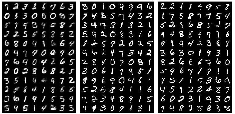
In a denoising auto encoder the goal is to create a more robust model to noise. The motivation is that the hidden layer should be able to capture high level representations and be robust to small changes in the input. The input of a DAE is noisy data but the target is the original data without noise:

$$\hat{\tilde{x}} = O(a(h) ) = Sigmoid ( c + w^{*} h(\tilde{x})),$$

$$h(\tilde{x}) = g(a(\tilde{x})) = Sigmoid (b + W\tilde{x}),$$

$$l = \frac{1}{2} \sum_{k=1}^N (x_{k} - \hat{\tilde{x_{k}}})^2$$

$$l = - \sum_{k=1}^N \big\{x_{k} log (\hat{\tilde{x}}_{k}) + (1 - x_{k}) log(1 - \hat{\tilde{x_{k}}})\big\}$$

Where $\tilde{x}$ is the noisy input. DAE can be used to denoise the input.

PyTorch Experiments (Github link)

Here is a PyTorch implementation of a DAE. To train a DAE, we can simply add some random noise to the data and create corrupted inputs. In this case 20% noise has been added to the input. The Fig3 shows the input ($x$), noisy input ($\tilde{x}$) and the reconstructed samples ($\hat{\tilde{x}}$) in the 200th epoch.

Fig3 - Denoising Autoencoders: From left to right: input, noisy input and output of the 200th epoch.
Fig4. DAE filters, the filters in a DAE show more distinctive features.

Variational Auto Encoders (VAE)

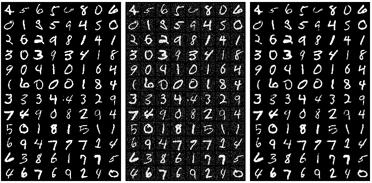
In a VAE, there is a strong assumption for the distribution that is learned in the hidden representation. The hidden representation is constrained to be a multivariate guassian. The motivation behind this is that we assume the hidden representation learns high level features and these features follow a very simple form of distribiution. Thus, we assume that each feature is a guassian distribiution and their combination which creates the hidden representation is a multivariate guassian.

From a probabilistic graphical models prespective, an auto encoder can be seen as a directed graphical model where the hidden units are latent variables ($z$) and the following rule applies:

$$p_{\theta}(x,\ z) = p_{\theta}(z)\ p_{\theta}(x|z),$$

where $\theta$ indicates that $p$ is parametrized by $\theta$. And according to the Bayes rule, the likelihood of the data ($p_{\theta}(x)$) can be derived using the following:

$$p_{\theta}(x) = \frac{p_{\theta}(x|\ z)\ p_{\theta}(z)}{p_{\theta}(z,\ x)},$$

$p_{\theta}(x|z)$ is the distribiution that generates the data ($x$) and is tractable using the dataset. In a VAE it is assumed the prior distribiution ($p_{\theta}(z)$) is a multivariate normal distribiution (centered at zero with co-varience of $I$):

$$p_{\theta}(z) = \prod_{k=1} ^ N \mathcal{N}(z_{k}\ |\ 0,1)$$

The posterior distribiution ($p_{\theta}(z|x)$) is an intractable distribiution (never observed), but the encoder learns $q_{\varphi}(z|x)$ as its estimator. As mentioned above, we assume $q_{\varphi}(z|x)$ is a normal distribiution which is parameterized by ${\varphi}$:

$$q_{\varphi}(z|x) = \prod_{k=1} ^ N \mathcal{N}(z_{k}\ |\ \mu_{k}(x),\ \sigma_{k}^2(x)).$$

Now the likelihood is parameterized by $\theta$ and $\varphi$. The goal is to find a $\theta^{*}$ and a $\varphi^{*}$ such that $log\ p_{\theta, \varphi}(x)$ is maximized. Or equivallently, we minimize the negative log-likelihood (nll):

In this setting, the following is a lower-bound on the log-likelihood of $x$. (Kingma and Welling, 2014.):

$$\mathcal{L}(x) = - D_{kl}\ (q_{\varphi}(z|x)\ ||\ p_{\theta}(z)) + E_{q_{\varphi}\ (z|x)}[\ log p_{\theta}(x\ |\ z)],$$

The second term is a reconstruction error which is approximated by sampling from
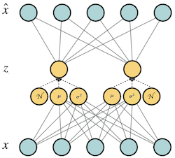
 $q_{\varphi}(z|x)$ (the encoder) and then computing $p_{\theta}(x\ |\ z)$ (the decoder). The first term, $D_{kl}$ is the Kullback–Leibler divergence which measures the differnce between two probability distribiutions. The KL term encourges the model to learn a $q_{\varphi}(z|x)$ that is of the form of $p_{\theta}(z)$ which is a normal distribiution and acts as a regularizer. Considering that $p_{\theta}(z)$ and $q_{\varphi}(z|x)$ are normal distribiutions, the KL term can be simplified to the following form:

$$ D_{kl}= \frac{1}{2}\ \sum_{k = 1}^{N}\ 1\ +\ log(\sigma_{k}^2 (x))- \mu_{k}^{2} (x) - \sigma_{k}^2 (x)$$
Fig5. Variational Auto Encoder: the hidden units parameterize the multivariate normal distribiution $q_{\varphi}(z|x)$ by finding a set of $(\ \mu,\ \sigma^2)$. $ \mathcal{N}$ is a normal distribiution from which we sample and is used in the reparametrization trick.

In short

A variational autoencoder has a very similar structure to an autoencoder except for several changes:

  • Strong assumption that the hidden representation follows a guassian distribiution.
  • The loss function has a new regularizer term (KL term) which forces the hidden representation to be close to a normal distribiution.
  • The model can be used for generation. Since the KL term makes sure that $q_{\varphi}(z|x)$ and $p_{\theta}(z)$ are close, one can sample from $q_{\varphi}(z|x)$ to generate new datapoints which will look very much like training samples.

The Reparametrization Trick

The problem that might come to ones mind is that how the gradient flows through a VAE where it involves sampling from
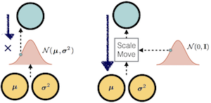
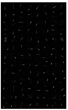
 $q_{\varphi}(z|x)$ which is a non-deterministic procedure. To tackle this problem, the reparametrization trick is used. In order to have a sample from the distribiution $ \mathcal{N}(\ \mu,\ \sigma^2)$, one can first sample from a normal distribiution $ \mathcal{N}(\ 0,\ 1)$ and then calculate:

$$ \mathcal{N}(\ \mu,\ \sigma^2) = \mathcal{N}(\ 0,\ 1) * \sigma^2 + \mu$$

Fig6. The reparametrization Trick: sampling from $ \mathcal{N}(\ \mu,\ \sigma^2)$ is non-deteministic and thus the gradient can not be passed through it. If one samples from the noraml distribiution $ \mathcal{N}(\ 0,\ 1)$ and just scale and move it using the parameters $\sigma^2,\ \mu$, the backward pass will be deterministic.

PyTorch Experiments (Github link)

Here is a PyTorch implementation of a VAE. The code also generates new samples. It also does a generation with interpolation which means that it starts from one sample and moves towards another sample in the latent space and generates new samples by interpolating between the mean and the variance of the first and second sample. Fig7. shows the generated samples with interpolation.
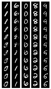
Fig7. From left to right: generated samples with interpolation at 1st, 40th, 80th, 150th and 200th epochs